Linear Regression

1. Closed Form source

We’d like to minimize the loss function, which in linear regression we use MSE:

Then we take the derivative, and get

which gives us:

As it takes a lot to calculate the inverse of $X^TX$, we can use pseudo inverse and matrix factorization instead.

2. Pseudo Inverse source1 source2 source3

By definition, pseudoinverse of matrix \(X^+=(X^TX)^{-1}X^T\). So if the $X$ is invertible, using pseudoinverse \(w=X^+y\) to calculate $w$ would be the same as the closed form.

• Note: in this case, to reduce the calculation cost, we can use singular vector decomposition \(X = UΣV^T\) to calculate \(X^+\), which is \(X^+ = 𝑉Σ^{−1}𝑈^T\). The \(Σ^{−1}\) is easy to compute if we just take the reciprocal of the diagnals.

When $X$ is not invertible, the pseudoinverse form would still work (in a pseudo way), which is better than the closed form. In this case, the diagnol of $Σ$ would have zero values. so \(X^+ = 𝑉Σ^{+}𝑈^T\), where the \(Σ^{+}\) would be taking the non-zero values’ reciprocal and keep the zero values zero.

The closed form would have $O(n^3)$ complexity while the SVD method would have $O(n^2)$ computational complexity.

3.GD, SGD, Mini-Batch GD

For regression problems, the loss function is convex. This means it will always have a global minimum.

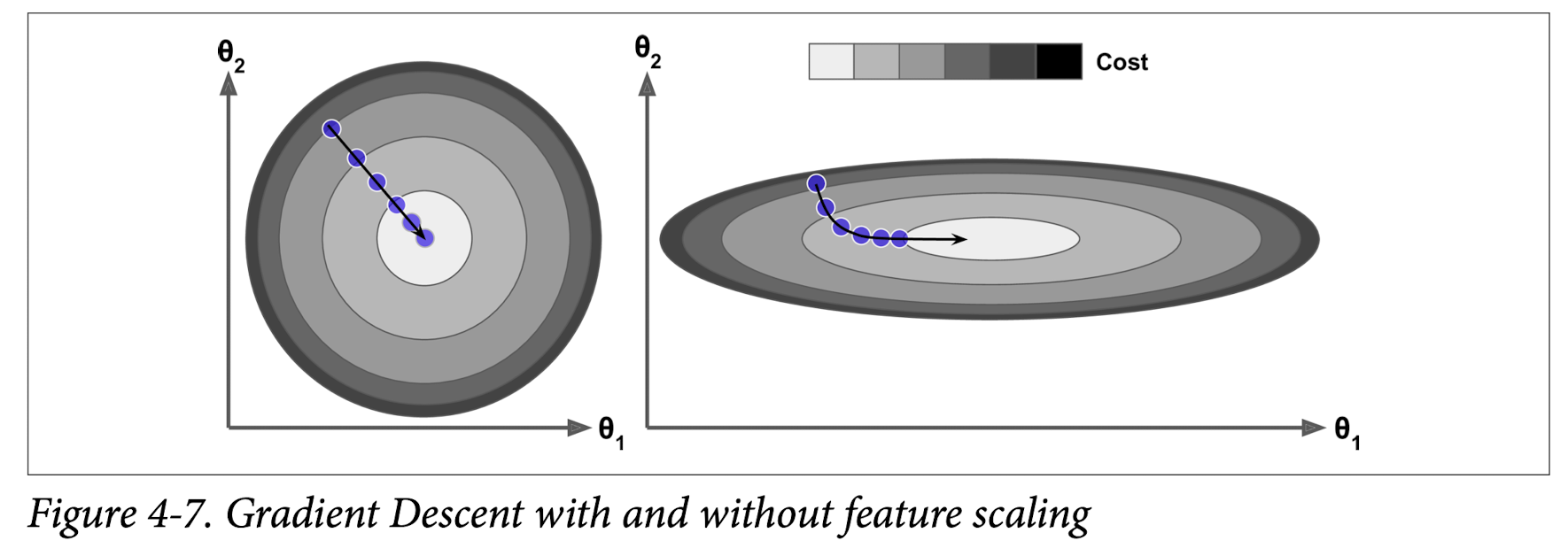
When we are using GD, we need to scale our data first, or the converging process would be longer. (if one feature is smaller, it would take a larger step to achieve similar decress in loss function as other features.)

We will calculate the gradient for each of the parameters, and take a step down.

• Note: the gradient is pointing uphill.

The SGD would take longer to reach global minimum, and bounce around it as new data point being added. But it allows the algorithm to jump out of local minimum and reach the global minimum.

**learning schedule**: If the learning rate is reduced too quickly, you may get stuck in a local minimum, or even end up frozen halfway to the minimum. If the learning rate is reduced too slowly, you may jump around the minimum for a long time and end up with a suboptimal solution if you halt training too early.

The training instances of SGD must be independent and identically distributed (IID)

If you do not do this, for example if the instances are sorted by label, then SGD will start by **optimizing for one label, then the next, and so on, and it will not settle close to the global minimum.**

4. Extension: Polynomial Regression

• Overfitting and underfitting
• Trade off between variance and bias

Regularized Linear Model

1. Ridge Regression

• regularization term: \(\alpha\sum^n\theta^2\), added to cost function. (It should not be added into evaluation function, as by objective, we aimed at decreasing the loss.)
• The bias term \(θ_0\) is not regularized.
• The input data need to be regularized.
• \[\hat θ=(X^TX+\alpha I)^{−1} X^T y\]

2. Lasso Regression

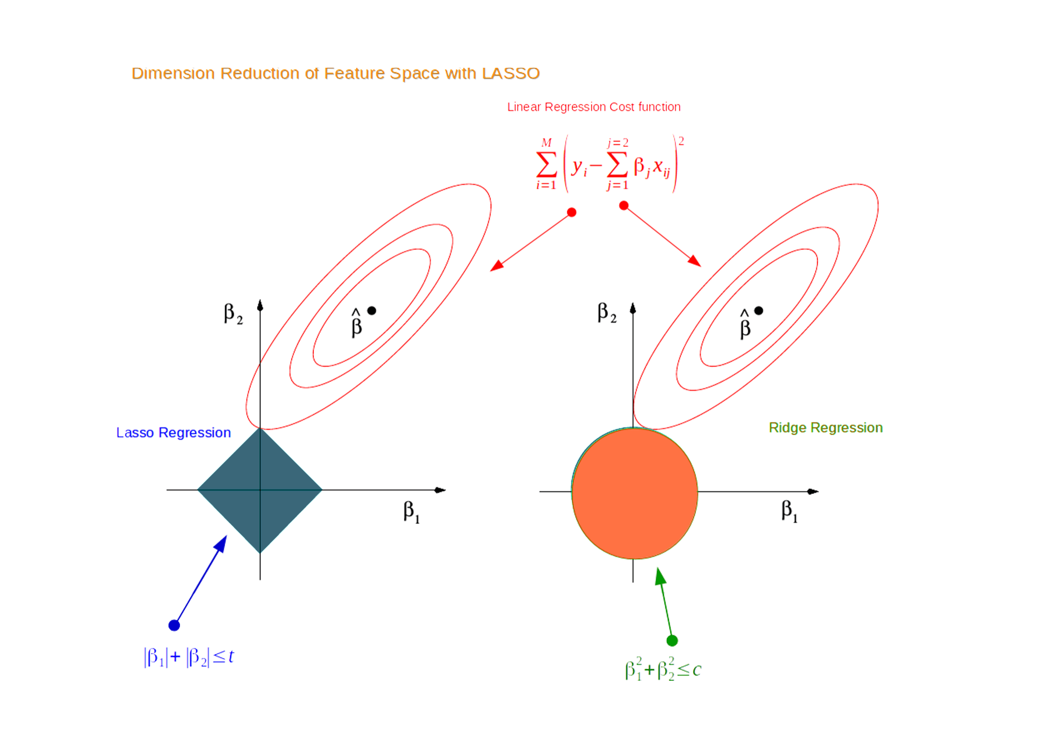
• regularization term: $$\alpha\sum^n

  \theta

  $$.

• Tends to completely elimi‐ nate the weights of the least important features, and return sparse outcome.
• \(\theta^T\theta = Constraint = C\), when \(\alpha\) goes up, \(C\) goes down.

For univariate linear regression or linear regression with uncorrelated features + lasso regularization, there is a closed-form solution. For more generalized forms of regression such as linear regression with correlated features or logistic regression, there is **no closed-form solution** of the lasso-regularized version. [Source](https://www.quora.com/Is-there-a-closed-form-solution-to-LASSO-regression)

3. Elastic Net

Combination of Ridge Regression and Lasso Regression.

Ridge is a good default, but if you suspect that only a few features are actually useful, you should **prefer Lasso or Elastic Net over ridge** since they tend to reduce the useless features’ weights down to zero as we have discussed. In general, **Elastic Net is preferred over Lasso** since Lasso may behave **erratically** when the number of features is greater than the number of training instances or when several features are **strongly correlated**.

4. Early Stopping

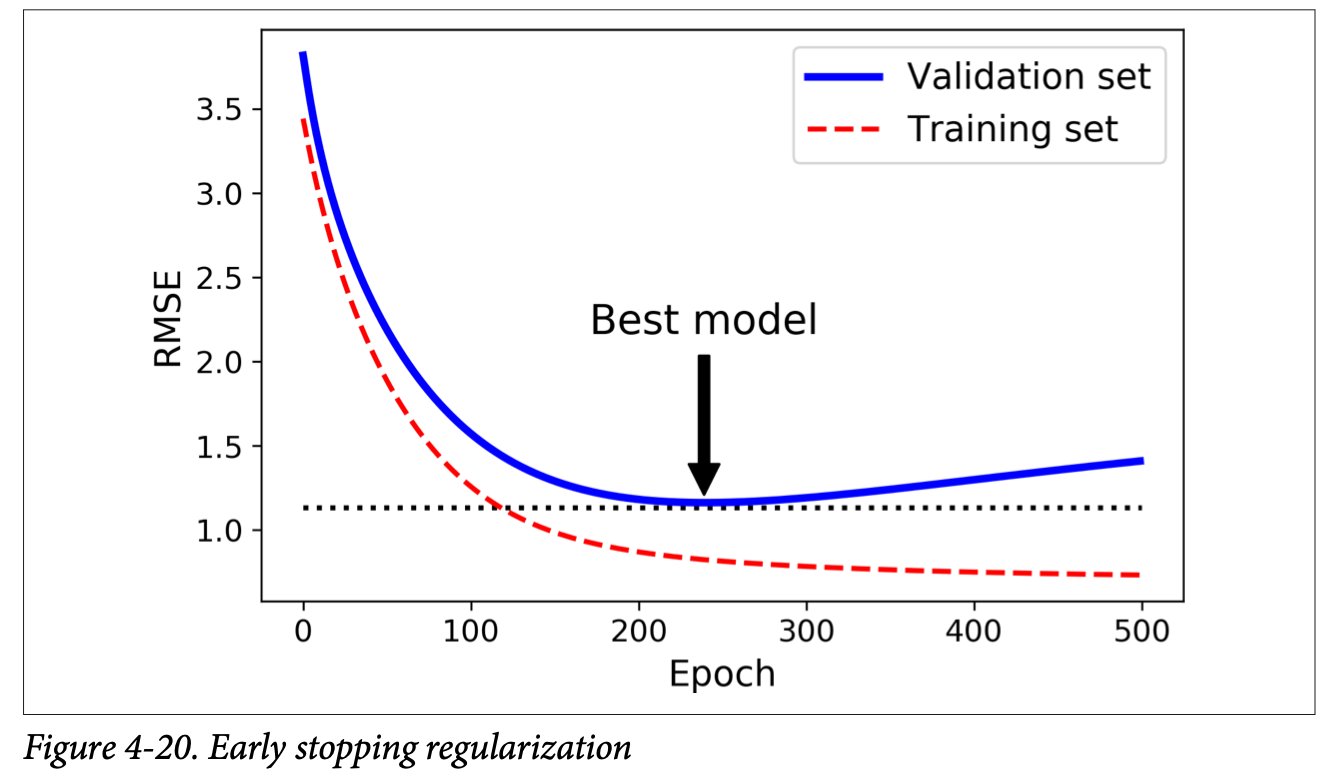
Using GD, and stop when validation error goes up. For SGD and Mini Batch, the curve would not be that smooth. So we can stop when validation error goes up for a while.

Logistic Regression

• Form: \(\hat p = \sigma(X^T\theta)\), where \(\sigma(t)=\frac{1}{1+exp^{-t}}\).

• t is called logit, \(logit(p)=log(\frac{p}{1-p})\),is the inverse of logistic function. \(t = logit(\hat p)\).

• Logit is also called log-odds, as it is the log of the ratio between the estimated probability for the positive class and the estimated probability for the negative class.

• MLE: \(likelihood = \hat y * y + (1 – \hat y) * (1 – y)\),

  • This function will always return a large probability when the model is close to the matching class value, and a small value when it is far away, for both y=0 and y=1 cases. Source

• log-likelihood = \(likelihood = log(\hat y) * y + log(1 – \hat y) * (1 – y)\)

  • equivalent to cross-entropy
  • Note: Cross entropy = \(-(log(q_{class0}) * p_{class0} + log(q_{class1}) * p_{class1})\)

• Cost function: \(log loss=-\frac{1}{m}\sum^m_{i=1}(y^ilog(\hat p^i)+(1-y^i)log(\hat (1-p^i)))\)

  • No closed form.

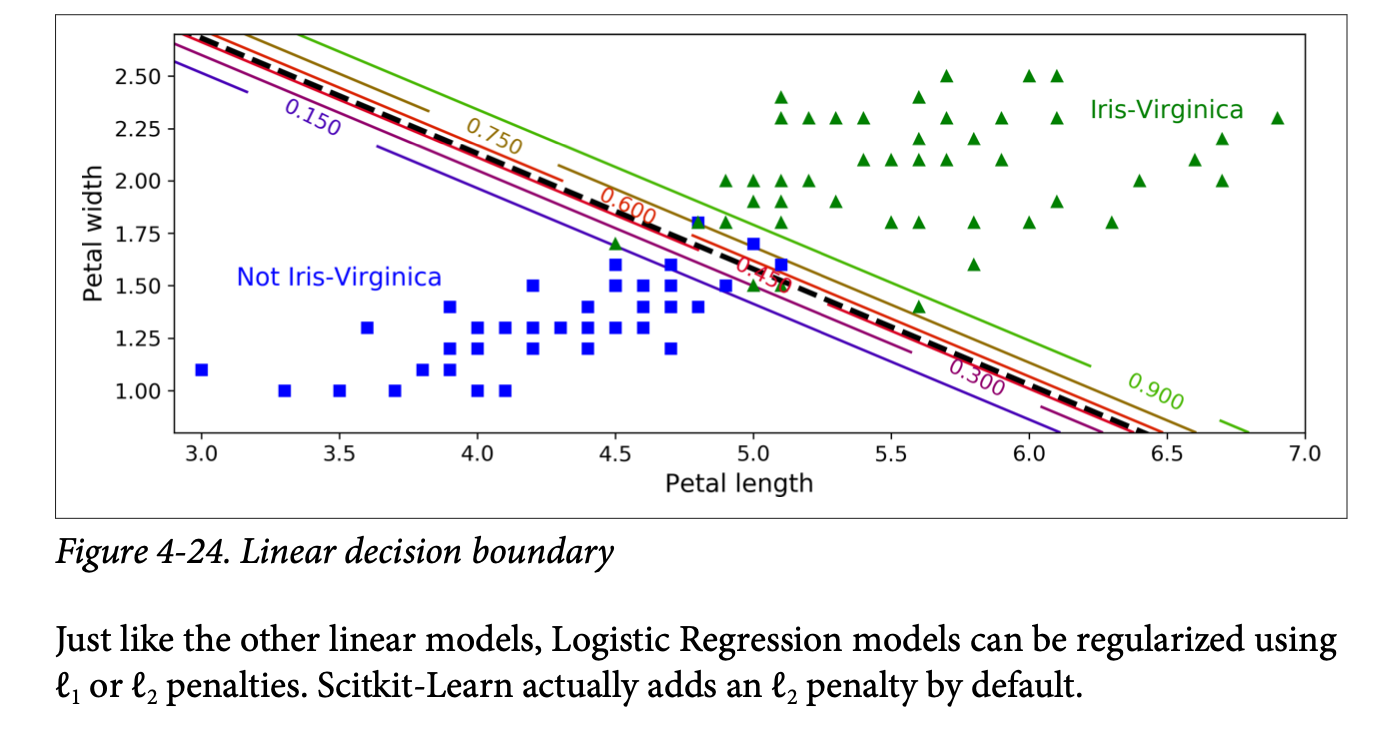
• Linear decision boundary

  • It is the the set of points x such that \(\theta_0 + \theta_1x_1 + \theta_2x_2 = 0\), which defines a straight line.

Softmax Regression

Softmax function: it computes the exponential of every score and normalizes them by dividing the sum of all the exponentials.