Support Vector Machine Math and Optimization
Math Basics
Duality
Optimization problems may be viewed from either of two perspectives, the primal problem or the dual problem. The solution to the dual problem provides a lower bound to the solution of the primal (minimization) problem In general the optimal values of the primal and dual problems need not be equal. Their difference is called the duality gap
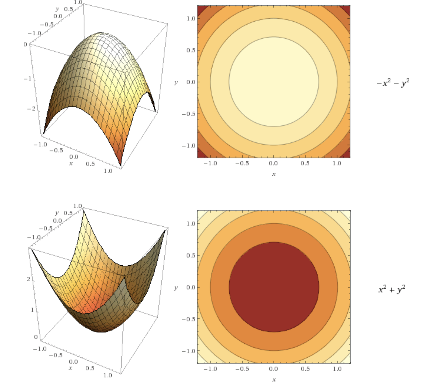
Contour lines
- For each point on a line, the function returns the same value
- The darker the area is, the smallest the value of the function is
Hyperplane
In geometry, a hyperplane is a subspace whose dimension is one less than that of its ambient space. For example, if a space is 3-dimensional then its hyperplanes are the 2-dimensional planes, while if the space is 2-dimensional, its hyperplanes are the 1-dimensional lines.
Lagrange multipliers
- Only works with equality constraints.
- The only one point where two vectors point in the same direction: it is the minimum of the objective function, under the constraint.
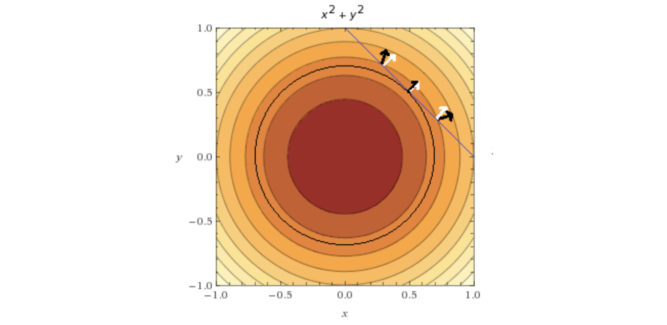
- Lagrange told us that to find the minimum of a constrained function, we need to look or points were \(\triangledown f(x,y)=\lambda \triangledown g(x,y)\).
- So we get \(\triangledown L(x,y,\lambda) = \triangledown f(x,y)-\lambda \triangledown g(x,y)\). The partial derivative of \(x,y,\lambda\) would all be zero.
Quadratic Programming
Perceptron Classifier
We’ll label the points into two labels {-1,1}, which gives us:
correct: \(y_{actual}*y_{predicted}>0\)
wrong: \(y_{actual}*y_{predicted}<0\)
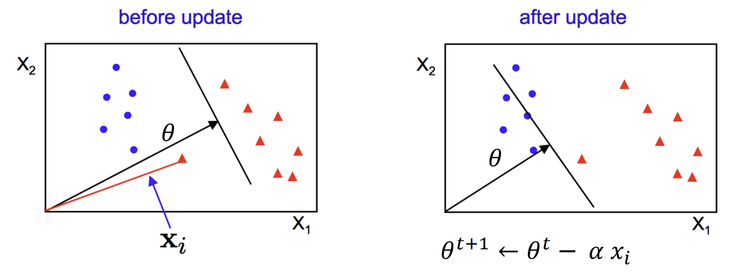
For two dimension:
\[\theta = (\theta_0,\theta_1,\theta_2)^T\\ x = (1,x_1,x_2)^T\\\]The decision boundary line we got would be:
\[\begin{aligned} \theta^T*x=0\\ \theta_0+\theta_1*x_1+\theta_2*x_2=0 \end{aligned}\]We’ll use iteration to find the line, for each missclassified point:
\[\theta_{updated}=\theta_{original}+\alpha*y_{actual}*x\]Linearly Seperable SVM
-
Two classes are linearly separable, SVM is to find the line that seperates the classes as far away as possible.
-
Support Vector: Any instance located on the “street”, including its border. The decision boundary is entirely determined by the support vectors.
-
SVM can output the confidence score by calculating the point’s distance from the decision boundary, byt there is no probability can be returned.
-
SVM is sensitive to feature scales. Or it will neglect the smaller feature.

- Hard margin classification: cannot deal with outliers. Thus we’ll use a more flexible model.
Math
| Step1: With normalization $$ | x_i \theta+b | = 1 \(, so the distance be\) \frac{1}{ | \theta | } $$ . |
Step2: We write down the primal form:
| Maximize $$\frac{1}{ | \theta | }$$ | ||
| Subject to min value of $$ | x_i\theta+b | $$ equals to 1 |
which could also be written as Minimize \(||\theta||=\frac{1}{2} \theta \theta^T\) Subject to \(|x_i\theta+b| \ge 1\)
Step3: We’d like to find the dual form. Using lagrange multiplier:
\[L(\theta,b,\alpha)=\frac{1}{2} \theta \theta^T - \Sigma^N_{i=1} \alpha_i( y_i(x_i\theta+b)-1)\]We take the partial derivative of \(\theta, b\), and get:
\[\theta = \Sigma^N_{i=1} \alpha_i y_i x_i\\ \Sigma^N_{i=1} \alpha_i y_i = 0\]Then we substitute the \(L(\theta,b,\alpha)\):
We need to maximize
\[\begin{aligned} L(\theta,b,\alpha) &= \Sigma^N_{i=1} \alpha_i+\frac{1}{2} \theta \theta^T -\Sigma^N_{i=1} \alpha_i y_i x_i\theta\\ &= \Sigma^N_{i=1} \alpha_i+\frac{1}{2}\Sigma^N_{i=1} \alpha_i y_i x_i \Sigma^N_{j=1} \alpha_j y_j x_j^T - \Sigma^N_{i=1} \alpha_i y_i x_i \Sigma^N_{j=1} \alpha_j y_j x_j^T \\ &=\Sigma^N_{i=1} \alpha_i -\frac{1}{2}\Sigma^N_{i=1}\Sigma^N_{j=1} \alpha_i \alpha_j y_i y_j x_i x_j^T \end{aligned}\]s.t. \(\alpha_i \ge 0\) and \(\Sigma^N_{i=1} \alpha_i y_i=0\)
As we can tell from the dual problem, the objective function now depends only on the Lagrange multipliers. Now we’ll use quadratic programming to solve for the best \(\alpha\).
Then for training, we get \(\theta=\Sigma^N_{i=1}\alpha_i y_i x_i\), b we pick any support vector and calculate \(y_i(x_i\theta+b)=1\).
For testing, we calculate \(s\theta+b=\Sigma\alpha_i y_i x_i s^T+b\) where \(s\) is (1*d) vector of testing point.
Not Linearly Separable SVM
Kernel Trick
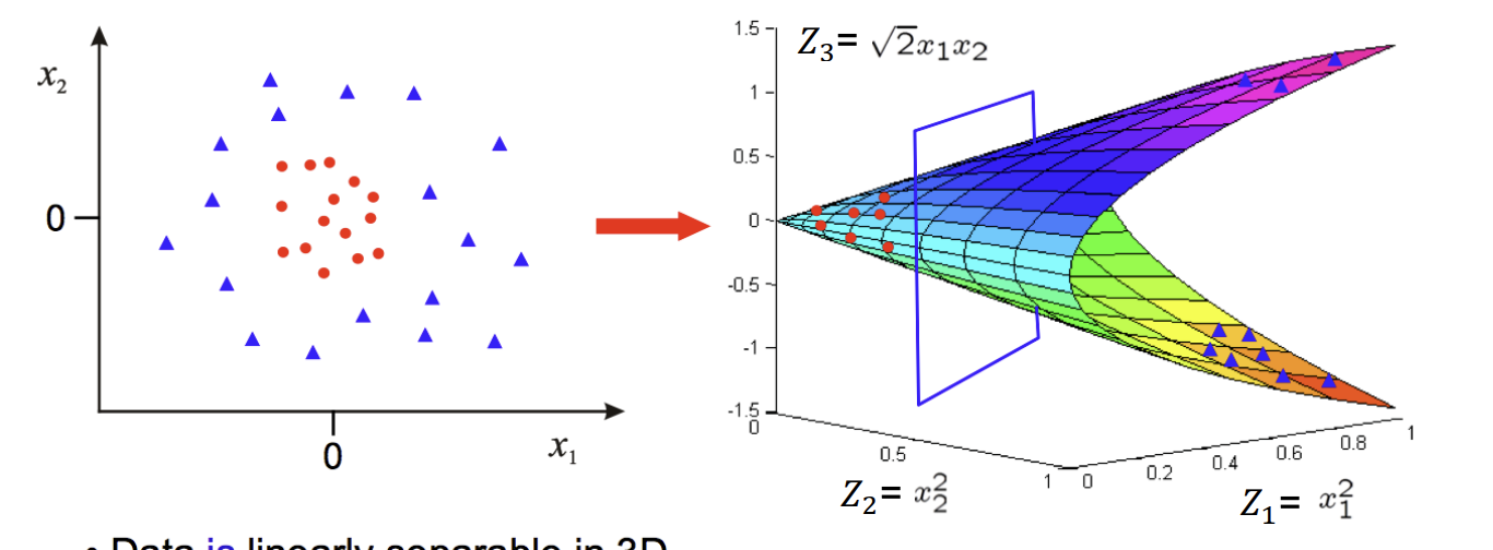
Idea 1: Use Polar Coordinates: for the “circle” seperable data, we can mapping the coordinate to polar coordinates.
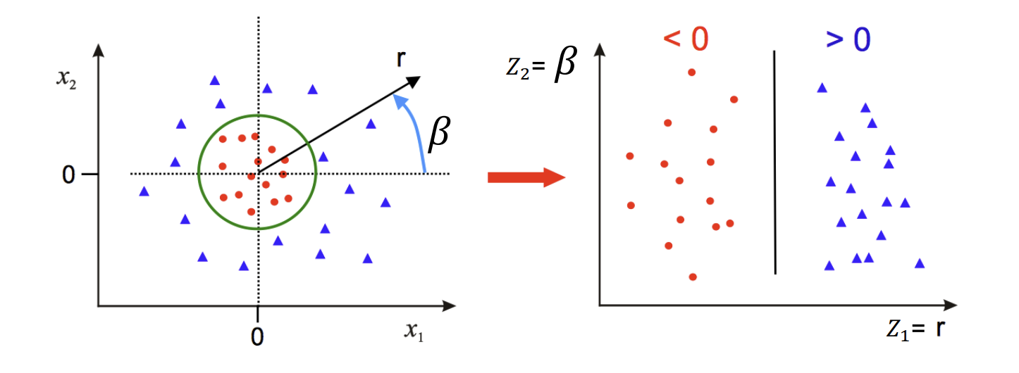
Map Data to Higher Dimension:
Common Kernels:
-
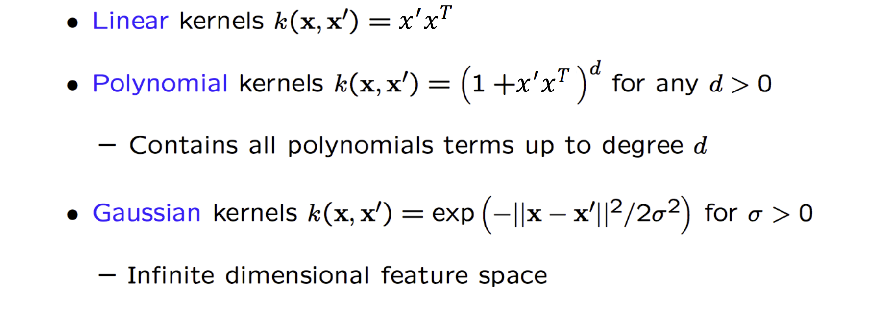
Always try the linear kernel first (remember that LinearSVC is much faster than SVC(ker nel=”linear”)), especially if the training set is very large or if it has plenty of features.
-
If the training set is not too large, you should try the Gaussian RBF kernel as well; it works well in most cases.
- The Gaussian RBF kernel has two hyperparameters: gamma: the higher, the narrower of the bell-shape curve, the more irregular of the decision boundary. C: The higher the narrower the street, thus less violation and higher irregular.
Soft Margin
We can penalize the violated points by adding:
Minimize \(\frac{1}{2} \theta \theta^T + C\Sigma^N_{i=1}\xi_i\) Subject to \(|x_i\theta+b| \ge 1-\xi_i\) Where \(\xi_i \ge 0\).
A smaller C value leads to a wider street but more margin violations
Complexity

- Gets dreadfully slow when the number of training instances gets large
- Perfect for complex but small or medium training sets, it scales well with the number of features, especially with sparse features (i.e., when each instance has few nonzero features).
- GD converges much more slowly than the methods based on QP.
- If there is millions of instances and a smaller number of features, it’s better to use primal form to optimize. The computational complexity of the primal form of the SVM problem is proportional tot he number of training instances m, while the comp. complexity of the dual form is proportional to a number between m^2 and m^3.source