Intro

Why Ensemble method?: Even if each classifier is a weak learner (meaning it does only slightly better than random guessing), the ensemble can still be a strong learner. Here are three types source:

• Bagging
• Boosting
• Stacking

Where to find a diverse set of classifiers?

• Use different training algorithm
• Use the same training algorithm for every predictor, but to train them on different random subsets of the training set.

How to aggregate?: Usually, we use Vote(take the statistical mode).

Bagging and Pasting

The aggregation function of Bagging and Pasting is typically the statistical mode. The difference is:

• Bagging: Sample with replacement
• Pasting: Sample without replacement

Pasting：

Similar to split the dataset into several subsets.

Bagging: Bootstrap aggregating

Given a standard training set \(D\) of size \(n\), bagging generates \(m\) new training sets \(D_{i}\), each of size \(n^′\), by sampling from D uniformly and with replacement.

By sampling with replacement, some observations may be repeated in each \(D_{i}\). If \(n^′=n\), then for large \(n\) the set \(D_{i}\) is expected to have the fraction \((1 - 1/e)≈63.2%\) of the unique examples of D, the rest being duplicates.

• Note: Each draw, the probability of not choosing that item is \((1−\frac{1}{n})\), if we draw \(n\) times, the probability of this item not being chosen would be \((1−\frac{1}{n})^n\). When \(n -> +\infty\)

Then, \(m\) models are fitted using the above \(m\) bootstrap samples and combined by averaging the output (for regression) or voting (for classification).

We usually use Bagging, because:

1. Bagging doesn’t require that big dataset
2. Bagging is less affected by the method of randomness (the pasting is similar to divide dataset into several subsets. The way we split the dataset matters.)

Note: Bootstrapping introduces a bit more diversity in the subsets that each predictor is trained on, so bagging ends up with a slightly higher bias than pasting, but this also means that predictors end up being less correlated so the ensemble’s variance is reduced.

The net result is that the ensemble has a similar bias but a lower variance than a single predictor trained on the original training set.

Bagging -> Random Forest

When training Random Forest, at each node only a random subset of the features is considered for splitting.

There are two parts of parameters need to be tuned. One is about trees characteristics; the other is about bagging process. Documentation

Tree-related

Random forest in sklearn is using CART decision tree, that is, for each node, we use Gini Index to split data. source

For decision trees, parameters are:

• max_depth int, default=None
  • The maximum depth of the tree. If None, then nodes are expanded until all leaves are pure or until all leaves contain less than min_samples_split samples. The min_samples_split is by default 2. So if we don’t set max_depth, the tree would split until there is only one sample data in the leaf.
• min_samples_split int or float, default=2
  • The minimum number of samples required to split an internal node:
• min_samples_leaf int or float, default=1
  • The minimum number of samples required to be at a leaf node.
• max_leaf_nodes int, default=None
  • Grow trees with max_leaf_nodes in best-first fashion. Best nodes are defined as relative reduction in impurity. If None then unlimited number of leaf nodes.
• min_impurity_decrease float, default=0.0
  • A node will be split if this split induces a decrease of the impurity greater than or equal to this value.
• max_features{“auto”, “sqrt”, “log2”}, int or float, default=”auto”
  • The number of features to consider when looking for the best split. For classification a good default is: m = sqrt(p)

Bagging-related

• n_estimators int, default=100
  • The number of trees in the forest.
• criterion {“gini”, “entropy”}, default=”gini”
• oob_score bool, default=False
  • Whether to use out-of-bag samples to estimate the generalization score. Only available if bootstrap=True.
• Bootstrap bool, default=True
  • Whether bootstrap samples are used when building trees. If False, the whole dataset is used to build each tree.
• max_samples int or float, default=None
  • If bootstrap is True, the number of samples to draw from X to train each base estimator

Boosting

Boosting is different from bagging in that the weak learners (in tree models, it would be CART trees) are sequentially built and correlated with each other. For Bagging, weak learners are independently built.

Adaboost

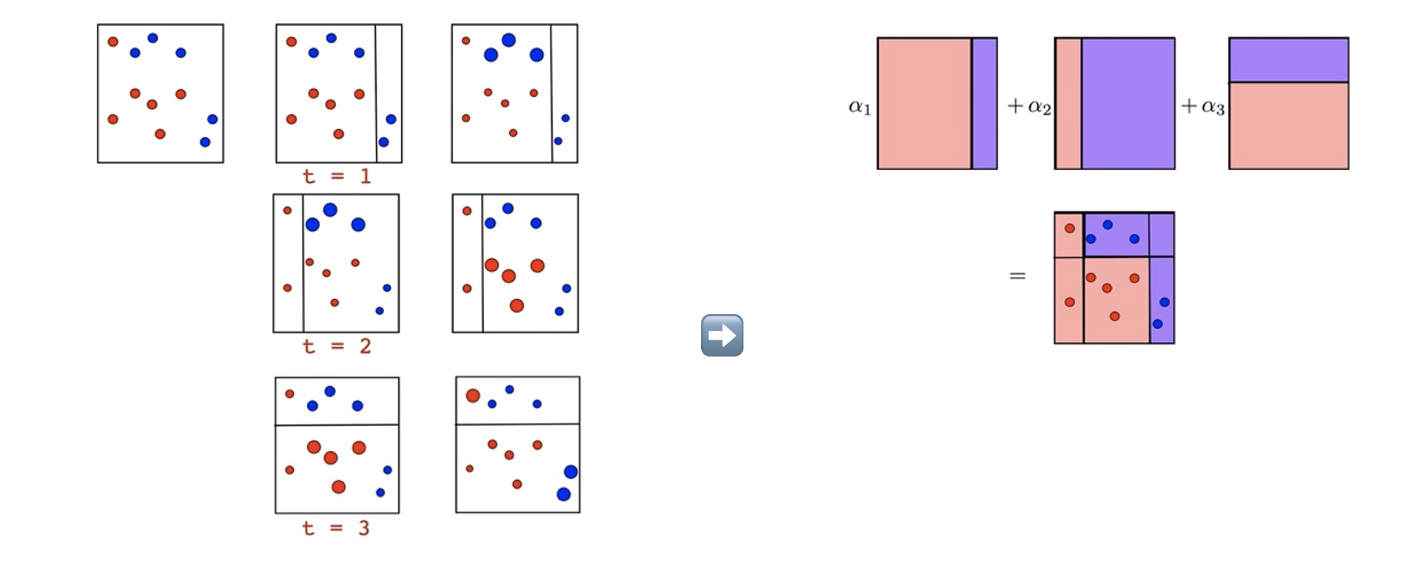
Adaboost was the first boosting algorithm, with a basic idea of sequentially building weak learners based on the former learner, assigning weights to those misclassified sample.

Once all predictors are trained, all predictors have different weights depending on their overall accuracy on the weighted training set, and we get the weighted sum of all predictors.

The weak learners in AdaBoost are decision trees with a single split, called decision stumps for their shortness.

Gradient Boosting

GB was brought up as a generalized version of Adaboost. It is to minimize the loss of the model by adding weak learners using a gradient descent like procedure.

Process:

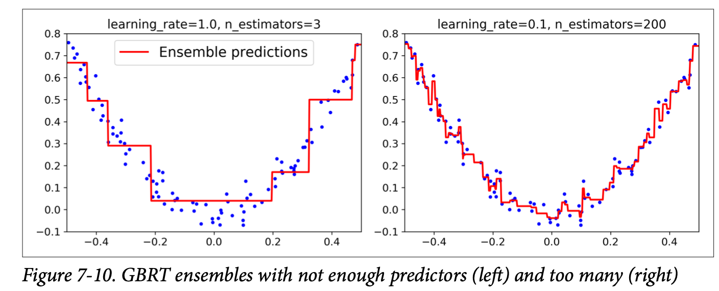
• The GB is to fit the new predictor to the residual errors made by the previous predictor
• After all the predictors were built, simply add up the predictions of all the trees.

Gradient boosting involves three elements:

1. A loss function to be optimized.
2. A weak learner to make predictions.
3. An additive model to add weak learners to minimize the loss function.

XGBoostmath, original paper

Important Advantagessource:

• Regularization:
  • Standard GBM implementation has no regularization like XGBoost, therefore it also helps to reduce overfitting.
  • Penalizes building complex tree with several leaf nodes
• Parallel Processing:
  • know more here
• Second derivative:
  • Gradient Boosting follows negative gradients to optimize the loss function, XGBoost uses Taylor expansion to calculate the value of the loss function for different base learners.

LightGBM source

Advanced version of XGBoost, has advantage in memory saving.

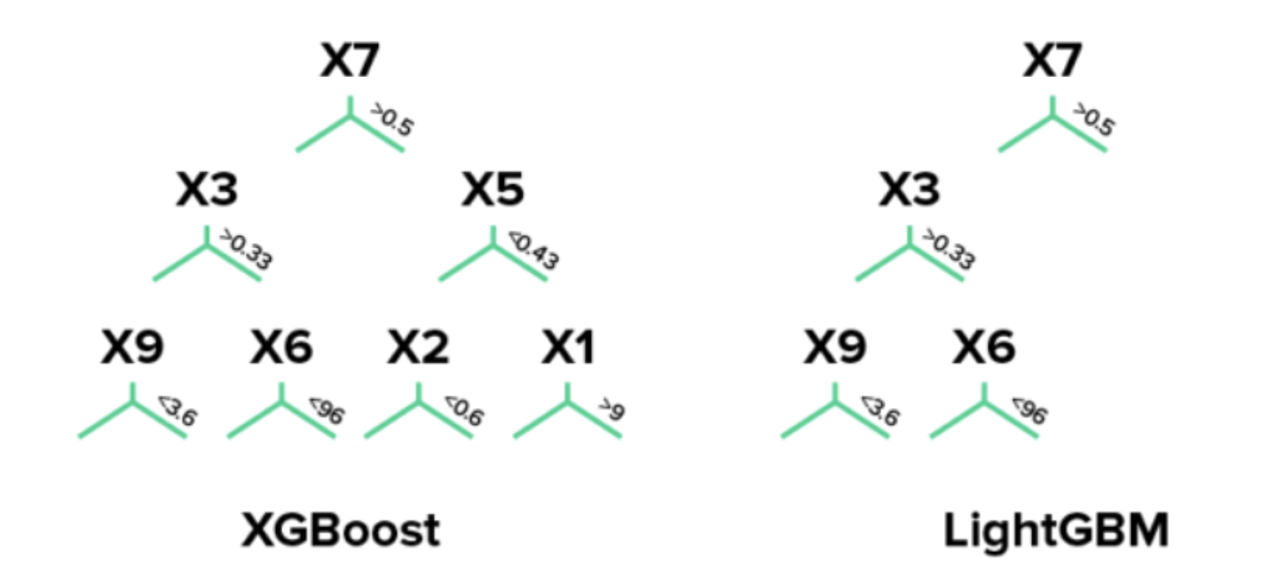
LightGBM uses leaf-wise (best-first) tree growth. It chooses to grow the leaf that minimizes the loss, allowing a growth of an imbalanced tree. Because it doesn’t grow level-wise, but leaf-wise, overfitting can happen when data is small. In these cases, it is important to control the tree depth.

XGboost splits up to the specified max_depth hyperparameter and then starts pruning the tree backwards and removes splits beyond which there is no positive gain. It uses this approach since sometimes a split of no loss reduction may be followed by a split with loss reduction. XGBoost can also perform leaf-wise tree growth (as LightGBM).

Stacking

Instead of using trivial functions (such as hard voting) to aggregate the predictions of all predictors in an ensemble, Stacking trains a model to perform this aggregation. The final predictor is called blender.

Step 1: the training set is split in two subsets. The first subset is used to train the predictors in the first layer

Step 2: the first layer predictors are used to make predictions on the second (held-out) set. We can create a new training set using these predicted values as input features, and keeping the target values.

Step 3: The blender is trained on this new training set, so it learns to predict the target value given the first layer’s predictions.

Feature Importance

Scikit-Learn measures a feature’s importance by looking at how much the tree nodes that use that feature reduce impurity on average (across all trees in the forest).

Impurity-based:

• impurity-based importances are biased towards high cardinality features;

• impurity-based importances are computed on training set statistics and therefore do not reflect the ability of feature to be useful to make predictions that generalize to the test set (when the model has enough capacity).

Permutation-based:

• overcomes limitations of the impurity-based feature importance: they do not have a bias toward high-cardinality features and can be computed on a left-out test set.

• The computation for full permutation importance is more costly.