Decision Tree Model - Advanced Review
Decision Tree
Key Takeaways
- No need to scale or center the data.
- Very likely to overfit the training data(not generalizing well).
- Very few assumptions about the training data( the data is non-linear). Non-parametric model: no assumptions about the shape of data.
- Effective learning with small training data, however very sensitive to small variations in the training data.
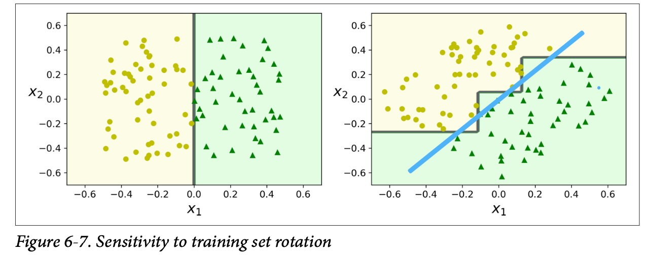
- Decision Boundary is irregular. Usually orthogonal decision boundaries.
- Probabilities: can return the class corresponding probability in the final tree node.
-
Missing value:
- ignoring the missing values
- treating the missing values as another category (in case of a nominal feature)
- all goes to the node which already has the biggest number of instances (CART, is not the primary rule)
- distribute to all children, but with diminished weights, proportional with the number of instances from each child node (C45 and others)
- Complexity, source: Training complexity: decision trees are generally approximately balanced, the number of node would be approximately \(O(log_2(m))\). Each node, we need to go through all the features and all the samples to calculate the split and impurity, which gives us complexity of \(O(nmlog_2(m))+O(nm) =>O(nmlog_2(m))\). (nmlogm is for sorting by each feature.O(nm) is going through each data point for each feature)(m is the number of samples,n is number of features.). Prediction complexity is just O(log2(m))
Training Algorithm
Gini Impurity
\[GiniIndex = 1-\Sigma p_i^2\]The i stands for class i. Gets its maximum value when the probability of the two classes is the same. The minimum value of Gini Index is 0, where the data is pure and only has one class.
Entropy
\[Entropy=–\Sigma p_i⋅log_2⋅p_i\]Gets its maximum value when the probability of the two classes is the same. Data is pure when the entropy has its minimum value, which is 0.
Gini vs. Entropy
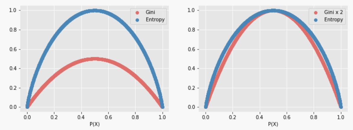
- Gini Index has values inside the interval [0, 0.5] whereas the interval of the Entropy is [0, 1].
- Computationally, entropy is more complex since it makes use of logarithms and consequently, the calculation of the Gini Index will be faster.
- Most of the time it does not make a big difference. However, when they differ, Gini impurity tends to isolate the most frequent class in its own branch of the tree, while entropy tends to produce slightly more balanced trees.

Calculation
Gini gain = \(Gini(Parent)\) - Weighted average of \(Gini(Child)\)
For each node, we choose the feature and threshold that have the most information gain.
Regularization
Hyperparameters Increasing min hyperparameters or reducing max hyperparameters will regularize the model.
- min_samples_split (the minimum number of samples a node must have before it can be split)
- min_samples_leaf (the minimum number of samples a leaf node must have)
- min_weight_fraction_leaf (same as min_samples_leaf but expressed as a fraction of the total number of weighted instances)
- max_leaf_nodes (maximum number of leaf nodes)
- max_features (maximum number of features that are evaluated for splitting at each node)
Pruning
Pruning processes can be divided into two types (pre- and post-pruning).
Pre-pruning procedures prevent a complete induction of the training set by replacing a stop () criterion in the induction algorithm (e.g. max. Tree depth or information gain (Attr)> minGain). Pre-pruning methods are considered to be more efficient because they do not induce an entire set, but rather trees remain small from the start. Prepruning methods share a common problem, the horizon effect. This is to be understood as the undesired premature termination of the induction by the stop () criterion.
Post-pruning (or just pruning) is the most common way of simplifying trees. Here, nodes and subtrees are replaced with leaves to reduce complexity. Pruning can not only significantly reduce the size but also improve the classification accuracy of unseen objects. It may be the case that the accuracy of the assignment on the train set deteriorates, but the accuracy of the classification properties of the tree increases overall.
The procedures are differentiated on the basis of their approach in the tree (top-down or bottom-up).
Bottom-up pruning These procedures start at the last node in the tree (the lowest point). Following recursively upwards, they determine the relevance of each individual node. If the relevance for the classification is not given, the node is dropped or replaced by a leaf. The advantage is that no relevant sub-trees can be lost with this method. These methods include Reduced Error Pruning (REP), Minimum Cost Complexity Pruning (MCCP), or Minimum Error Pruning (MEP).
Top-down pruning In contrast to the bottom-up method, this method starts at the root of the tree. Following the structure below, a relevance check is carried out which decides whether a node is relevant for the classification of all n items or not. By pruning the tree at an inner node, it can happen that an entire sub-tree (regardless of its relevance) is dropped. One of these representatives is pessimistic error pruning (PEP), which brings quite good results with unseen items.
A node whose children are all leaf nodes is considered unnecessary if the purity improvement it provides is not statistically significant.
- Reduced error pruning (source:tamu.edu, cs663)
- Classify examples in validation set
- For each node:
- Sum the errors over entire subtree
- Calculate error on same example if converted to a leaf with majority class label
- Prune node with highest reduction in error
- Repeat until error no longer reduced
- For each node:
- Cost complexity pruning
- Significant testing
The \(\chi^2\) test: estimate the probability that the improvement is purely the result of chance (which is called the null hypothesis)
Regression
The main difference is that regression tree split the training set in a way that minimizes the MSE. The predicted value for each region is always the average target value of the instances in that region.
\[J(k, t_k) = \frac{m_{left}}{m} MSE_{left} + \frac{m_{right}}{m} MSE_{right}\]where:
\[MSE_{node}=\Sigma(\hat y_{node}-y^{i})^2\\ \hat y_{node}=\frac{1}{m_{node}}\Sigma y^{i}\]Limitation and Methods
1. Overfitting
2. Orthogonal decision boundaries
cannot generalized well when the ground truth of decision boundary has slope. One way is to use PCA first.

3. Sparse features
Not designed to work with very sparse features. When data is sparse, decision trees overfit. Can use PCA.
4. Unstable source
A small change in the dataset can make the tree structure unstable which can cause variance.
5. Imbalanced data
Reading: Using Random Forest to Learn Imbalanced Data
Decision tree learners create underfit trees if some classes are imbalanced. It is therefore recommended to balance the data set prior to fitting with the decision tree. source
The splitting process is always done through gini or entropy and therefore always maximises accuracy - the only way you can influence F1 or AUC on a single tree would be through finding the subtree that optimizes those via postpruning, or to choose the hyperparameters of the ensambling procedure. Therefore yes - standard trees do not handle unbalanced classes, but some optimization around can.source
We can use Weighted Gini (or Entropy) to take into account the class distribution, or using a mixture of Under and Over sampling of the classes when bagging decision trees.source
All the following based on source
- Class weight
- simply provide a weight for each class which places more emphasis on the minority classes such that the end result is a classifier which can learn equally from all classes.
- in tree based model, decreased entropy to determine how to split the data, can simply scale the entropy component of each class by the corresponding weight such that you place more emphasis on the minority classes.
- In a gradient-based model, place more significance on the losses associated with minority classes.
-
Oversampling
- Randomly sample the minority classes and simply duplicate the sampled observations.(but is also artificially reducing the variance of the dataset)
- Synthetic Minority Over-sampling Technique (SMOTE) is a technique that generates new observations by interpolating between observations in the original dataset.
- a new (synthetic) observation is generated by interpolating between one of the k-nearest neighbors, xzi.
- Adaptive Synthetic (ADASYN) sampling works in a similar manner as SMOTE, however, the number of samples generated for a given xi is proportional to the number of nearby samples which do not belong to the same class as xi. Thus, ADASYN tends to focus solely on outliers when generating new synthetic training examples.
-
Undersampling
- Random undersampling
- could potentially result in removing key characteristics of the majority class.
- Near miss
- only the sample the points from the majority class necessary to distinguish between other classes.
- N farthest samples and N nearest samples
- Random undersampling
- Remove vague data points
- Tomek’s link
- Edited nearest neighbors